Visualising London rental bike location data
⋅ 15 minute read ⋅ 3,019 words
Contents
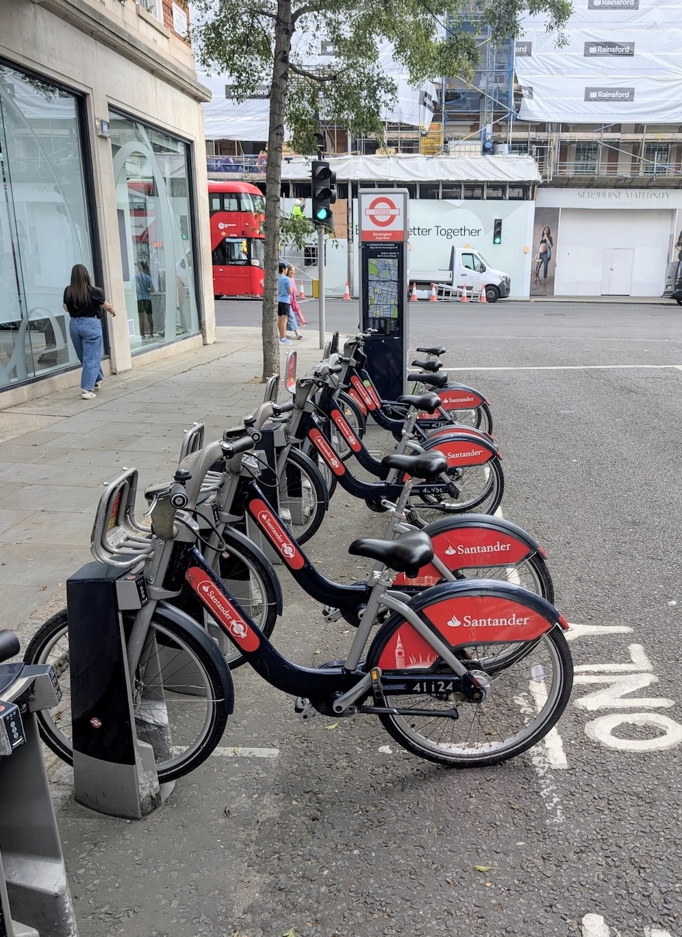
London has a great rental bike scheme that makes it easy to get around the city. Rather than free-floating you can rent bikes from fixed bike stations like the one shown below. If you get the yearly membership you even get a key that you can use to rent the bike without an app.
Image(filename='map_images/station_photo.jpg', width='400px')
Moreover, Transport for London makes the live rental station data available on this endpoint . I collected hourly snapshots of bike availability data over a month so I can play around with it with DuckDB’s new spatial features and QGIS.
§Collecting the data
I created a simple script fetch_bike_data.sh and a cronjob on a Hetzner VPS to request and store the data every hour. Here is the script:
#!/bin/bash
DATE=\\((date +"%Y.%m.%d.%H.%M.%S")
DIR=/home/projects/bike\_data

mkdir -p \\)DIR
curl -o santander.$DATE.xml https://tfl.gov.uk/tfl/syndication/feeds/cycle-hire/livecyclehireupdates.xml
After adding permissions to the script with chmod +x fetch_bike_data.sh I modify crontab:
crontab -eand add the following line to run this script:
0 * * * * /home/projects/bike_data/fetch_bike_data.shEach request is stored to an XML-file on disk which has the following format:
<stations lastUpdate="1784031061002" version="2.0">
    <station>
        <id>1</id>
        <name>River Street , Clerkenwell</name>
        <terminalName>001023</terminalName>
        <lat>51.52916347</lat>
        <long>-0.109970527</long>
        <installed>true</installed>
        <locked>false</locked>
        <installDate>1278947280000</installDate>
        <removalDate/>
        <temporary>false</temporary>
        <nbBikes>0</nbBikes>
        <nbStandardBikes>0</nbStandardBikes>
        <nbEBikes>0</nbEBikes>
        <nbEmptyDocks>19</nbEmptyDocks>
        <nbDocks>19</nbDocks>
    </station>
    <station>
        <id>2</id>
        <name>Phillimore Gardens, Kensington</name>
        <terminalName>001018</terminalName>
        <lat>51.49960695</lat>
        <long>-0.197574246</long>
        <installed>true</installed>
        <locked>false</locked>
        <installDate>1278585780000</installDate>
        <removalDate/>
        <temporary>false</temporary>
        <nbBikes>6</nbBikes>
        <nbStandardBikes>6</nbStandardBikes>
        <nbEBikes>0</nbEBikes>
        <nbEmptyDocks>28</nbEmptyDocks>
        <nbDocks>37</nbDocks>
    </station>
[...]
As you can see the raw data contains per-station information about its name, location, and bike availability.
§Convert to DuckDB table
I load and combine all the XML-files into a DuckDB database london_bike_data so that I can use SQL to analyse it. Before I do that I install the extensions spatial and h3 for the geospatial features and webbed to read xml files.
import duckdb
from IPython.display import Image

# Connect to DuckDB
conn = duckdb.connect('london_bike_data.duckdb')

conn.execute("INSTALL spatial;")
conn.execute("INSTALL h3 FROM community;")
conn.execute("INSTALL webbed FROM community;")
conn.execute("LOAD spatial;")
conn.execute("LOAD h3;")
conn.execute("LOAD webbed;");
The next query loads all collected xml-files into one DuckDB table and enforces the schema, adds metadata, and handles missing data issues. Note the Hetzner instance was based in Helsinki which I account for when converting the filename into a timestamp with the correct time zone.
conn.execute("""
    CREATE OR REPLACE TABLE londonbikestations AS
     SELECT
            strptime(
            regexp_extract(filename, 'santander\\.(\\d{4}\\.\\d{2}\\.\\d{2}\\.\\d{2}\\.\\d{2}\\.\\d{2})\\.xml', 1),
            '%Y.%m.%d.%H.%M.%S'
        ) AT TIME ZONE 'Europe/Helsinki' AT TIME ZONE 'Europe/London' AS downloaded_at,
                 id::INTEGER AS id,
                 name,
                 terminalName AS terminal_name,
                 lat::DOUBLE AS lat,
                 long::DOUBLE AS lng,
                 installed::BOOLEAN AS installed,
                 locked::BOOLEAN AS locked,
                 temporary::BOOLEAN AS temporary,
                 nbBikes::INTEGER AS nb_bikes,
                 nbStandardBikes::INTEGER AS nb_standard_bikes,
                 nbEBikes::INTEGER AS nb_ebikes,
                 nbEmptyDocks::INTEGER AS nb_empty_docks,
                 nbDocks::INTEGER AS nb_docks,
                epoch_ms(installDate::BIGINT) AS install_date,
                CASE WHEN removalDate = '' THEN NULL ELSE epoch_ms(removalDate::BIGINT) END AS removal_date
             FROM read_xml('data/santander.*.xml', all_varchar=true, filename=true)
""")
conn.sql("select count(*) from londonbikestations")
┌──────────────┐
│ count_star() │
│ int64 │
├──────────────┤
│ 707197 │
└──────────────┘
The query below shows the station data that is available. The table contains the station id, name and coordinates (lat, lng) and when it was installed and/or removed. For every station I have the capacity nb_docks and the current number of rentable bikes nb_bikes (split into standard and ebikes).
conn.sql("describe table londonbikestations")┌───────────────────┬─────────────┬─────────┬─────────┬─────────┬─────────┐
│ column_name │ column_type │ null │ key │ default │ extra │
│ varchar │ varchar │ varchar │ varchar │ varchar │ varchar │
├───────────────────┼─────────────┼─────────┼─────────┼─────────┼─────────┤
│ downloaded_at │ TIMESTAMP │ YES │ NULL │ NULL │ NULL │
│ id │ INTEGER │ YES │ NULL │ NULL │ NULL │
│ name │ VARCHAR │ YES │ NULL │ NULL │ NULL │
│ terminal_name │ VARCHAR │ YES │ NULL │ NULL │ NULL │
│ lat │ DOUBLE │ YES │ NULL │ NULL │ NULL │
│ lng │ DOUBLE │ YES │ NULL │ NULL │ NULL │
│ installed │ BOOLEAN │ YES │ NULL │ NULL │ NULL │
│ locked │ BOOLEAN │ YES │ NULL │ NULL │ NULL │
│ temporary │ BOOLEAN │ YES │ NULL │ NULL │ NULL │
│ nb_bikes │ INTEGER │ YES │ NULL │ NULL │ NULL │
│ nb_standard_bikes │ INTEGER │ YES │ NULL │ NULL │ NULL │
│ nb_ebikes │ INTEGER │ YES │ NULL │ NULL │ NULL │
│ nb_empty_docks │ INTEGER │ YES │ NULL │ NULL │ NULL │
│ nb_docks │ INTEGER │ YES │ NULL │ NULL │ NULL │
│ install_date │ TIMESTAMP │ YES │ NULL │ NULL │ NULL │
│ removal_date │ TIMESTAMP │ YES │ NULL │ NULL │ NULL │
└───────────────────┴─────────────┴─────────┴─────────┴─────────┴─────────┘
16 rows 6 columns
The removal_date column seems not trustworthy since there is definitely activity (changes in nb_bikes) happening at stations that have a removal date, e.g.
conn.sql("select downloaded_at, name, terminal_name, nb_bikes, removal_date from londonbikestations where terminal_name = '000968' order by downloaded_at")┌─────────────────────┬──────────────────────────┬───────────────┬──────────┬─────────────────────┐
│ downloaded_at │ name │ terminal_name │ nb_bikes │ removal_date │
│ timestamp │ varchar │ varchar │ int32 │ timestamp │
├─────────────────────┼──────────────────────────┼───────────────┼──────────┼─────────────────────┤
│ 2026-05-08 22:00:01 │ Warwick Row, Westminster │ 000968 │ 6 │ 2018-10-18 06:56:00 │
│ 2026-05-08 23:00:01 │ Warwick Row, Westminster │ 000968 │ 6 │ 2018-10-18 06:56:00 │
│ 2026-05-09 00:00:01 │ Warwick Row, Westminster │ 000968 │ 6 │ 2018-10-18 06:56:00 │
│ 2026-05-09 01:00:01 │ Warwick Row, Westminster │ 000968 │ 6 │ 2018-10-18 06:56:00 │
│ 2026-05-09 02:00:01 │ Warwick Row, Westminster │ 000968 │ 6 │ 2018-10-18 06:56:00 │
│ 2026-05-09 03:00:01 │ Warwick Row, Westminster │ 000968 │ 6 │ 2018-10-18 06:56:00 │
│ 2026-05-09 04:00:01 │ Warwick Row, Westminster │ 000968 │ 6 │ 2018-10-18 06:56:00 │
│ 2026-05-09 05:00:01 │ Warwick Row, Westminster │ 000968 │ 6 │ 2018-10-18 06:56:00 │
│ 2026-05-09 06:00:01 │ Warwick Row, Westminster │ 000968 │ 6 │ 2018-10-18 06:56:00 │
│ 2026-05-09 07:00:01 │ Warwick Row, Westminster │ 000968 │ 6 │ 2018-10-18 06:56:00 │
│ · │ · │ · │ · │ · │
│ · │ · │ · │ · │ · │
│ · │ · │ · │ · │ · │
│ 2026-06-14 12:00:01 │ Warwick Row, Westminster │ 000968 │ 3 │ 2018-10-18 06:56:00 │
│ 2026-06-14 13:00:01 │ Warwick Row, Westminster │ 000968 │ 5 │ 2018-10-18 06:56:00 │
│ 2026-06-14 14:00:01 │ Warwick Row, Westminster │ 000968 │ 9 │ 2018-10-18 06:56:00 │
│ 2026-06-14 15:00:01 │ Warwick Row, Westminster │ 000968 │ 4 │ 2018-10-18 06:56:00 │
│ 2026-06-14 16:00:01 │ Warwick Row, Westminster │ 000968 │ 2 │ 2018-10-18 06:56:00 │
│ 2026-06-14 17:00:01 │ Warwick Row, Westminster │ 000968 │ 7 │ 2018-10-18 06:56:00 │
│ 2026-06-14 18:00:01 │ Warwick Row, Westminster │ 000968 │ 9 │ 2018-10-18 06:56:00 │
│ 2026-06-14 19:00:01 │ Warwick Row, Westminster │ 000968 │ 10 │ 2018-10-18 06:56:00 │
│ 2026-06-14 20:00:01 │ Warwick Row, Westminster │ 000968 │ 11 │ 2018-10-18 06:56:00 │
│ 2026-06-14 21:00:01 │ Warwick Row, Westminster │ 000968 │ 8 │ 2018-10-18 06:56:00 │
└─────────────────────┴──────────────────────────┴───────────────┴──────────┴─────────────────────┘
887 rows (20 shown) 5 columns
I have confirmed that this station still exists ( here ) so I will just ignore this column.
I want to get an overview of the total capacity across all stations. The exact number fluctuates slightly between snapshots but the capacity seems to be around 20.9k. The maximum number of docked bikes was 7708 standard bikes and 1131 eBikes. The official numbers given by TfL are 10,000 standard bikes and 2,000 eBikes.
conn.sql("select downloaded_at, sum(nb_standard_bikes) as sum_docked_standard_bikes, sum(nb_ebikes) as sum_docked_ebikes, sum(nb_docks) as sum_station_capacity from londonbikestations group by downloaded_at order by sum_docked_standard_bikes")┌─────────────────────┬───────────────────────────┬───────────────────┬──────────────────────┐
│ downloaded_at │ sum_docked_standard_bikes │ sum_docked_ebikes │ sum_station_capacity │
│ timestamp │ int128 │ int128 │ int128 │
├─────────────────────┼───────────────────────────┼───────────────────┼──────────────────────┤
│ 2026-06-04 08:00:01 │ 6008 │ 795 │ 20963 │
│ 2026-06-01 08:00:01 │ 6047 │ 585 │ 20934 │
│ 2026-06-03 08:00:01 │ 6056 │ 948 │ 20951 │
│ 2026-06-02 08:00:01 │ 6082 │ 927 │ 20921 │
│ 2026-06-04 17:00:01 │ 6122 │ 1185 │ 20963 │
│ 2026-06-09 08:00:02 │ 6127 │ 830 │ 20962 │
│ 2026-05-28 08:00:01 │ 6191 │ 692 │ 20950 │
│ 2026-06-01 17:00:01 │ 6201 │ 1086 │ 20892 │
│ 2026-05-27 17:00:01 │ 6203 │ 829 │ 20950 │
│ 2026-06-04 10:00:01 │ 6210 │ 983 │ 20963 │
│ · │ · │ · │ · │
│ · │ · │ · │ · │
│ · │ · │ · │ · │
│ 2026-05-16 06:00:01 │ 7668 │ 1081 │ 20969 │
│ 2026-05-15 01:00:01 │ 7671 │ 1182 │ 20949 │
│ 2026-05-15 03:00:01 │ 7674 │ 1169 │ 20949 │
│ 2026-05-16 01:00:01 │ 7678 │ 1172 │ 20942 │
│ 2026-05-15 02:00:01 │ 7678 │ 1178 │ 20949 │
│ 2026-05-16 00:00:01 │ 7679 │ 1186 │ 20942 │
│ 2026-05-16 02:00:01 │ 7699 │ 1157 │ 20942 │
│ 2026-05-16 05:00:01 │ 7703 │ 1106 │ 20969 │
│ 2026-05-16 03:00:01 │ 7705 │ 1143 │ 20942 │
│ 2026-05-16 04:00:01 │ 7708 │ 1131 │ 20942 │
└─────────────────────┴───────────────────────────┴───────────────────┴──────────────────────┘
887 rows (20 shown) 4 columns
The largest station is Jubilee Plaza in Canary Wharf.
conn.sql("select name, nb_bikes, nb_docks from londonbikestations order by nb_docks desc limit 1")┌─────────────────────────────┬──────────┬──────────┐
│ name │ nb_bikes │ nb_docks │
│ varchar │ int32 │ int32 │
├─────────────────────────────┼──────────┼──────────┤
│ Jubilee Plaza, Canary Wharf │ 42 │ 63 │
└─────────────────────────────┴──────────┴──────────┘
§Busiest stations
To approximate the busiest stations I sum the absolute hour-to-hour change in nb_bikes per station. This approximates total churn (bikes leaving and arriving) since simultaneous arrivals and departures within the same hour cancel out.
conn.execute("""
    CREATE OR REPLACE TABLE busy_stations AS
    WITH hourly_changes AS (
        SELECT
            terminal_name,
            ST_POINT(lng, lat) AS geometry,
            name,
            downloaded_at,
            nb_bikes,
            abs(nb_bikes - lag(nb_bikes) OVER w) AS abs_change
        FROM londonbikestations
        WINDOW w AS (PARTITION BY terminal_name ORDER BY downloaded_at)
    )
    SELECT
        terminal_name,
        geometry,
        any_value(name) AS name,
        sum(abs_change) AS total_churn,
        count(*) AS nb_snapshots
    FROM hourly_changes
    GROUP BY terminal_name, geometry
    ORDER BY total_churn DESC
""")
conn.sql("""select name, total_churn from busy_stations limit 20""")
┌──────────────────────────────────────────┬─────────────┐
│ name │ total_churn │
│ varchar │ int128 │
├──────────────────────────────────────────┼─────────────┤
│ Hop Exchange, The Borough │ 3218 │
│ Soho Square , Soho │ 3160 │
│ Argyle Street, Kings Cross │ 2930 │
│ Waterloo Station 2, Waterloo │ 2753 │
│ Hyde Park Corner, Hyde Park │ 2605 │
│ Waterloo Station 1, Waterloo │ 2554 │
│ Moorfields, Moorgate │ 2527 │
│ Brushfield Street, Liverpool Street │ 2514 │
│ Waterloo Station 3, Waterloo │ 2389 │
│ St. James's Square, St. James's │ 2360 │
│ Jubilee Plaza, Canary Wharf │ 2289 │
│ Eagle Wharf Road, Hoxton │ 2263 │
│ Cheapside, Bank │ 2202 │
│ Imperial College, Knightsbridge │ 2181 │
│ Worship Street, Shoreditch │ 2167 │
│ Natural History Museum, South Kensington │ 2142 │
│ Whitehall Place, Strand │ 2042 │
│ Queen's Gate (North), Kensington │ 2019 │
│ Malet Street, Bloomsbury │ 2013 │
│ Exhibition Road, Knightsbridge │ 1987 │
└──────────────────────────────────────────┴─────────────┘
20 rows 2 columns
None of these stations are surprising. As we can see later on the map all of these stations are in the city centre or close to commuter train stations.
§Busiest hours of the day
Using the same total-churn metric I group the data by hour of day to see when bike activity peaks.
conn.sql("""
    WITH hourly_changes AS (
        SELECT
            terminal_name,
            downloaded_at,
            nb_bikes,
            abs(nb_bikes - lag(nb_bikes) OVER w) AS abs_change
        FROM londonbikestations
        WINDOW w AS (PARTITION BY terminal_name ORDER BY downloaded_at)
    )
    SELECT
        hour(downloaded_at) AS hour_of_day,
        sum(abs_change) AS total_churn,
        count(*) AS nb_snapshots
    FROM hourly_changes
    GROUP BY hour_of_day
    ORDER BY total_churn
""")
┌─────────────┬─────────────┬──────────────┐
│ hour_of_day │ total_churn │ nb_snapshots │
│ int64 │ int128 │ int64 │
├─────────────┼─────────────┼──────────────┤
│ 3 │ 3911 │ 29501 │
│ 4 │ 4111 │ 29501 │
│ 2 │ 5398 │ 29501 │
│ 5 │ 7441 │ 29502 │
│ 1 │ 8518 │ 29501 │
│ 0 │ 13462 │ 29501 │
│ 6 │ 20333 │ 29502 │
│ 23 │ 21172 │ 29500 │
│ 22 │ 29554 │ 29500 │
│ 21 │ 33808 │ 28702 │
│ · │ · │ · │
│ · │ · │ · │
│ · │ · │ · │
│ 13 │ 40336 │ 29497 │
│ 20 │ 40433 │ 29499 │
│ 10 │ 41575 │ 29495 │
│ 7 │ 45237 │ 29503 │
│ 19 │ 47598 │ 28707 │
│ 16 │ 54813 │ 29498 │
│ 9 │ 57626 │ 29498 │
│ 17 │ 64213 │ 29498 │
│ 18 │ 64873 │ 30300 │
│ 8 │ 78166 │ 29503 │
└─────────────┴─────────────┴──────────────┘
24 rows (20 shown) 3 columns
We see the highest activity from 7:00-8:00, 8:00-9:00, 16:00-17:00, 17:00-18:00 which are peak commuter hours and the lowest activity in the early morning.
§Storing geometric data as parquet files
Before I can use QGIS for map-based visualisations I need to store the relevant data in a compatible format.
I want to show the number of bikes available across the city at different times of the day (I picked Wednesday 27.5.2026). To aggregate the number of available bikes spatially, I group by H3 cells . If the coordinates of the bike station fall into the cell I sum all available bikes.
conn.execute("""
    CREATE OR REPLACE TABLE bike_station_geo AS
        SELECT *, ST_POINT(lng, lat) AS geometry FROM londonbikestations where downloaded_at::date = '2026-05-27'
""")
conn.execute("""
    CREATE OR REPLACE TABLE h3_cell_covering AS
        SELECT
            downloaded_at,
            H3_LATLNG_TO_CELL(
                ST_Y(geometry),
                ST_X(geometry),
                7
            ) AS hexagon,
            sum(nb_bikes) AS nb_bikes
        FROM bike_station_geo
        GROUP BY 1, 2
""");
I then store the h3 bike counts table as a parquet file. This involves conversion of the hexagon data into WKB(well-known-binary) that GeoParquet uses to store geometries. Note: By default the geometry in DuckDB is assumed to be EPSG:4326.
conn.execute("""
COPY (
      SELECT geometry: ST_ASWKB(H3_CELL_TO_BOUNDARY_WKT(hexagon)::geometry),
              date_trunc('hour', downloaded_at) AS downloaded_at,
             nb_bikes
      FROM   h3_cell_covering
  ) TO 'available_bikes_per_h3_7_cell.parquet';
  """);
I also want to visualise the location of the busy stations on the map, so I store the busy stations as a separate file.
conn.execute("""
COPY (
      SELECT *  FROM busy_stations
  ) TO 'busy_stations.parquet';
""");§Visualising availability using QGIS
QGIS (3.44.10) is an open-source geographic information system. It allows combining, viewing, and analysing tabular data with geographic and mapping data.
I want to display our parquet data over an actual map of London. To get this map, I install the plugin NextGIS MapServices and then restart QGIS to make it available. I use OpenStreetMap as the base map. In the toolbar click on QuickMapService(Globe icon) and add the OpenstreetMap OSM Standard. Next, in Project Properties (Cmd+Shift+P)-> CRS change the Projection or Coordinate Reference System to EPSG:3857 (Pseudo-Mercator).
§Visualising busy stations
Drag and drop the busy_stations.parquet file into the Layers field (bottom left). Ensure under Layer Properties –> Assigned Coordinate Reference System that EPSG:4326 - WGS 84 is selected. This allows QGIS to correctly reproject the geography data from the file onto the map.
Under Layer Properties –> Symbology I can change the style of the location marker to show all the stations. You can see all the coordinates of stations in the dataset below.
Image(filename='map_images/station_locations.jpg')
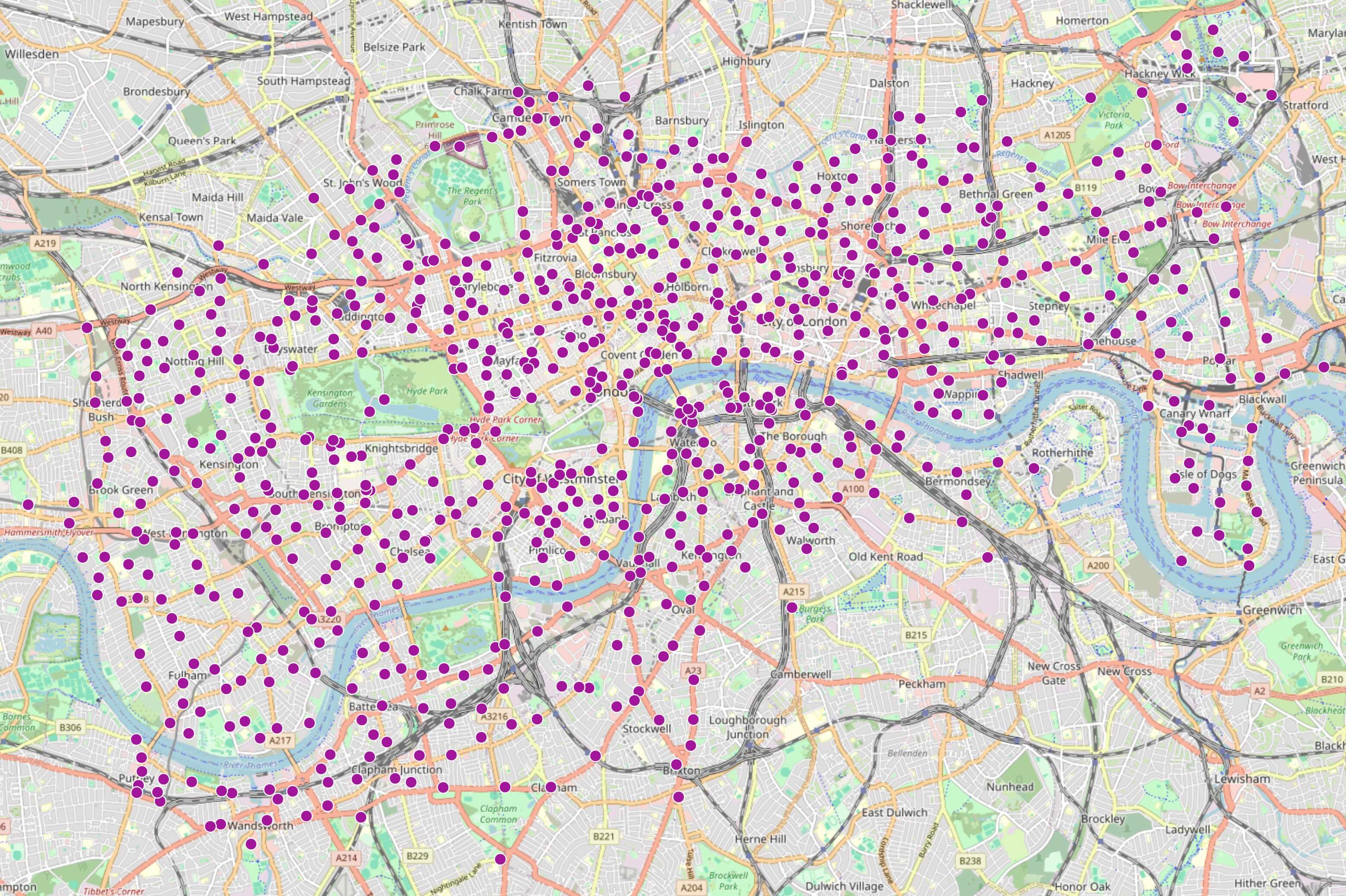
To only show the top 20 busiest stations as calculated in the previous section I add a filter on the busy stations layer. (Right click on layer –> Filter, then add total_churn > 1900). I also want to show the station names, so I go to Layer Properties –> Label –> Single labels and select for value the Expression Builder and then use the expression: "name" || ' (' || to_string("total_churn") || ')' to concatenate the churn value to the station name in brackets.
Image(filename='map_images/busy_stations.jpg')
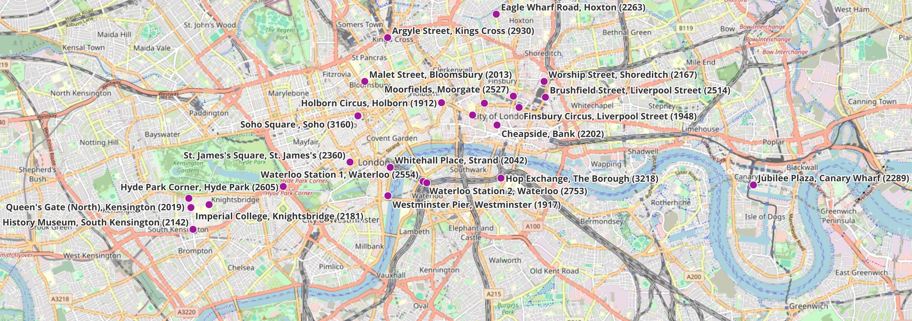
Unsurprisingly the busiest stations are in the centre where many Londoners work (Bank, Canary Wharf, Soho, Westminster) or close to major train stations (Liverpool Street, King’s Cross, Waterloo, Hop Exchange).
§Rental bike availability during commute hours
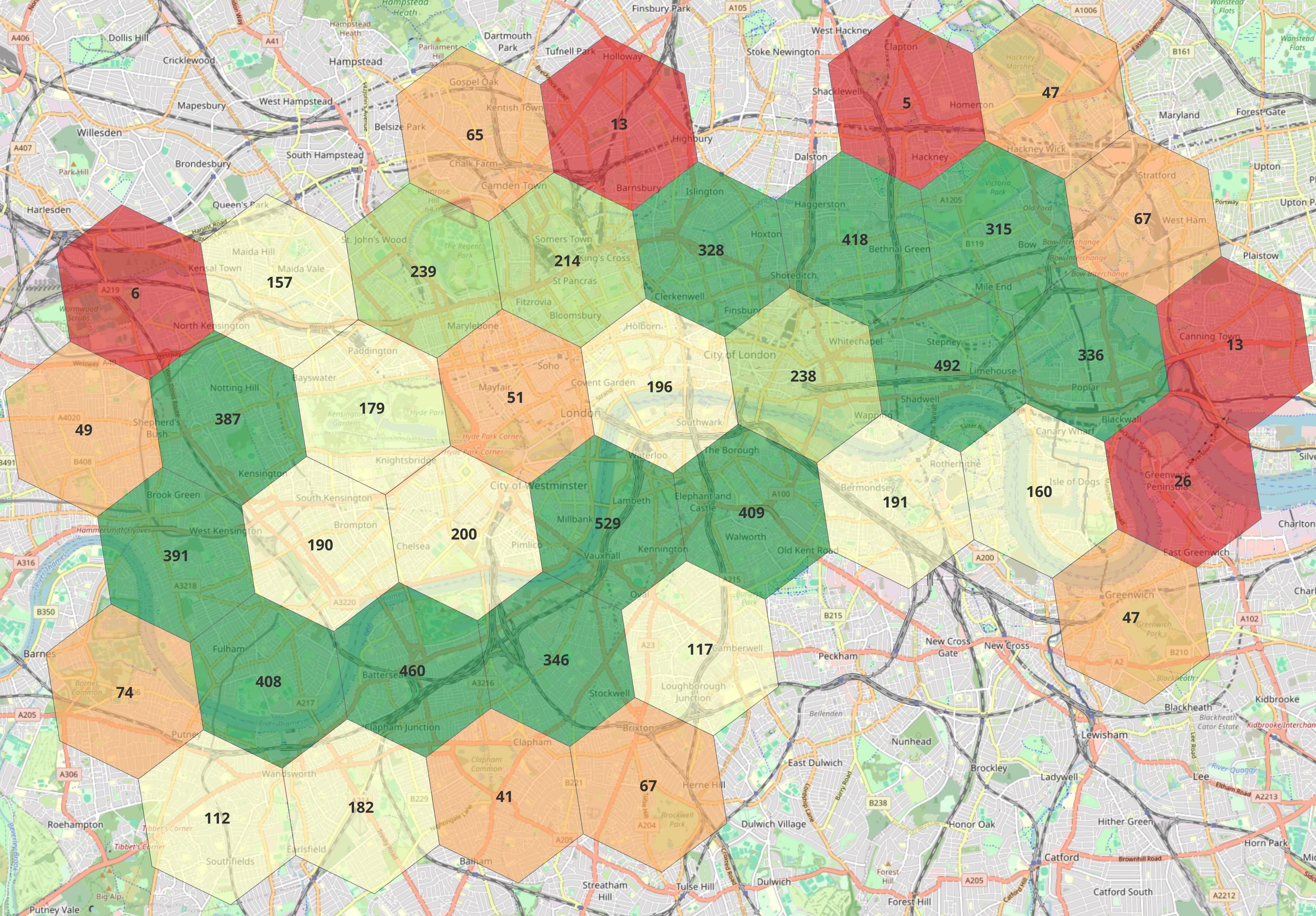
I also want to visualise how the rental bikes move before and after morning rush hour. My expectation is that fewer bikes are initially in the city centre (zone 1) and more bikes in the outer residential areas (zones 2 and 3). Then around 11am we should see a concentration of bikes in zone 1.
I drag and drop the relevant data file available_bikes_per_h3_7_cell.parquet to create a new Layer. Again, I first ensure that the projection for this dataset is set to EPSG:4326 - WGS 84. The hexagons should now appear on top of the map. Remember that the file has availability data for every hour of the day, so I add a Layer filter: "downloaded_at" = '2026-05-27T06:00:00.000' to only use data from one point in time before the start of the rush hour.
To style the hex fields according to the number of available bikes in the hexagon area I make the following changes in the Layer properties:
Symbology–>Graduated–> Value:nb_bikes, Color Ramp:RdYlGr, Mode:Equal Interval, Opacity:60%Labels–>Single Labels–> Value:nb_bikes, 18Pt, Bold.
I have filtered the layer once for 6am and once for 11am and here are the two outputs:
display(Image(filename='map_images/bike_availibility_6am.jpg'))
display(Image(filename='map_images/bike_availibility_11am.jpg'))
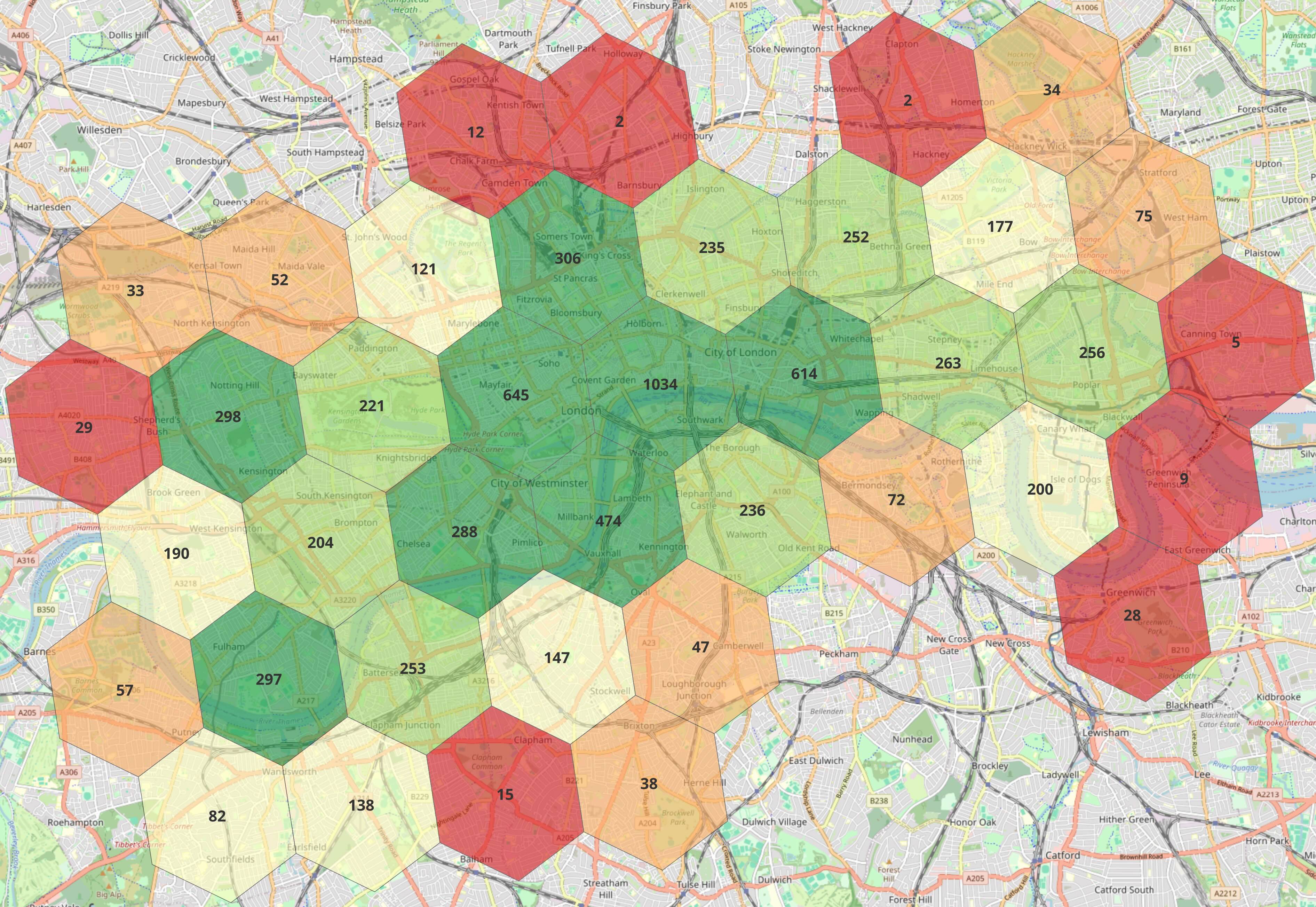
As expected you can see that a lot of the residential districts along the water, West Kensington, Fulham, Wandsworth, Battersea, Elephant and Castle and in the east around Limehouse, Mile End, Bethnal Green see an outflow of available bikes. The central districts around the City of London, Mayfair, King’s Cross and Westminster accumulate a lot of the bikes by 11am.
§Conclusion
It turns out to be pretty easy to collect, explore and visualise the London bike station data. DuckDB makes it really easy to ingest hundreds of XML files and the H3 and spatial extensions allow easy geographical aggregation. This is my first time using QGIS. It took 20min to get up to speed with it, but it’s really cool how it fuses mapping data and geographical and analytical data. I will try to use it in other projects as well.
§References
- I was inspired by Mark Litwintschik’s ebike fleet monitoring blog post
- A useful QGIS Tutorial is available here
§Jupyter Notebook
You can find the Jupyter notebook and the datasets for this post here .
If you have any thoughts, questions, or feedback about this post, I would love to hear it. Please reach out to me via email.
#data-engineering #data-science #duck-db #qgis